Geothermal Case Study

ESMDA example predicting temperature at a production well as a function of permeability.

This example demonstrates the application of the Ensemble Smoother with Multiple Data Assimilation (ESMDA) using the dageo library to predict temperature at a production well in a geothermal reservoir. The notebook integrates the Delft Advanced Research Terra Simulator (DARTS) to model the impact of permeability variations on temperature over a 30-year period. The example uses a channelized permeability field, which provides an interesting case study of ESMDA’s behavior with non-Gaussian geological features. Since ESMDA operates under Gaussian assumptions, it tends to create smooth updates to the permeability field rather than maintaining sharp channel boundaries. This limitation becomes particularly visible when the algorithm identifies the need for connectivity between wells - instead of creating or modifying channels, it increases permeability in a more diffuse manner. This behavior highlights both the power of ESMDA in matching production data and its limitations in preserving complex geological features.

Tip

This example can serve as an example how one can use dageo with any external modelling code, here with the Delft Advanced Research Terra Simulator (DARTS).

Thanks to Mona Devos, who provided the initial version of this example!

Pre-computed data

DARTS computation

The DARTS computation in this example takes too long for it to be run automatically on GitHub with every commit for the documentation (CI). We therefore pre-computed the results locally to show them here. You can change the flag compute_darts from False to True to actually compute the results with DARTS yourself. The pre-computed results were generated with the following versions (taking roughly 4 h on a single thread):

• open-darts: 1.1.4

• Python: 3.10.15

• NumPy: 2.0.2

• SciPy: 1.14.1

Fluvial models

The fluvial models were generated with FLUVSIM through geomodpy, for more information see towards the end of the example where the code is shown to reproduce the facies.

Important

To retrieve the pre-computed data (for both DARTS and the facies), you need to have pooch installed:

pip install pooch

or

conda install -c conda-forge pooch

import pooch
import numpy as np
import matplotlib.pyplot as plt

import dageo

compute_darts = False
if compute_darts:
    from darts.engines import redirect_darts_output
    from darts.models.darts_model import DartsModel
    from darts.physics.geothermal.physics import Geothermal
    from darts.reservoirs.struct_reservoir import StructReservoir
    from darts.physics.geothermal.property_container import PropertyContainer

    redirect_darts_output("run_geothermal.log")

    # For reproducibility, we instantiate a random number generator with a
    # fixed seed. For production, remove the seed!
    rng = np.random.default_rng(42)

Load pre-computed data

folder = "data"
ffacies = "facies_geothermal.npy"
fdarts = "darts_output_geothermal.npz"

# Load Facies: Not needed if you compute the facies yourself,
#              as described at the end of the notebook.
fpfacies = pooch.retrieve(
    "https://raw.github.com/tuda-geo/data/2024-11-30/resmda/"+ffacies,
    "9b18f1c80aea93d7973effafde001aa7e72a21ac91edf08e3899d5486998ad2e",
    fname=ffacies,
    path=folder,
)
facies = np.load(fpfacies)

# Load pre-computed DARTS result; only needed if `compute_darts=False`.
if not compute_darts:
    fpdarts = pooch.retrieve(
        "https://raw.github.com/tuda-geo/data/2024-11-30/resmda/"+fdarts,
        "5622729cd5dc7214de8a199512ace39bda48bff113b2eddb0c48593a57c020d1",
        fname=fdarts,
        path=folder,
    )
    pc_darts = np.load(fpdarts)

Convert facies to permeability

Here we define some model parameters. Important: These have obviously to agree with the facies you computed!

# Model parameters
nx, ny, nz = 60, 60, 3   # 60 x 60 x 3 cells
dx, dy, dz = 30, 30, 30  # Each cell is a voxel of 30 x 30 x 30 meter
ne = 100                 # 100 ensembles
years = np.arange(31)    # Time: we are modelling 30 years:

# Well locations
iw = [30, 30]
jw = [14, 46]

# Minimum and maximum values for permeability
perm_min = 100.
perm_max = 200.

# Get permeability fields by populating the facies
perm = np.zeros(facies.shape)
perm[facies == 0] = perm_min  # outside channels minimum
perm[facies > 0] = perm_max   # inside channels maximum

# We use a model with 3 layers, starting all with the same permeability.
perm = np.stack([perm]*nz, axis=-1)  # 3x the same

# Assign true permeability (first) and prior permeability
perm_true = perm[:1, :, :, :]
perm_prior = perm[1:, :, :, :]

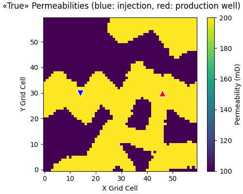
Plot “true” model

The true permeability model is the one facies realization we use to create observations by adding noise to the modelled data. These observations are what we try to match with ESMDA. To look at this permeability field is important to later interpret the result. In particular, we see that there is a channel of high permeability connecting the injection with the production well.

fopts = {"sharex": True, "sharey": True, "constrained_layout": True}
popts = {"vmin": perm_min, "vmax": perm_max, "origin": "lower"}

fig, ax = plt.subplots(figsize=(5, 4), **fopts)

# Permeabilities
im = ax.imshow(perm_true[0, :, :, 0], **popts)

# Wells
ax.plot(jw[0], iw[0], "v", c="b", ms=10, mec="w")
ax.plot(jw[1], iw[1], "^", c="r", ms=10, mec="w")

# Labels and colour bar
ax.set_ylabel("Y Grid Cell")
ax.set_xlabel("X Grid Cell")
fig.suptitle(
    "«True» Permeabilities (blue: injection, red: production well)"
)
cbar = fig.colorbar(im, ax=ax, label="Permeability (mD)")

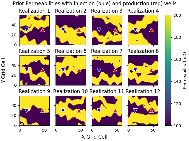
Prior permeabilities

Plot the first 12 prior permeability models; yellow shows the channels with higher permeability.

fig, axs = plt.subplots(3, 4, **fopts)

for i, ax in enumerate(axs.ravel()):
    ax.set_title(f"Realization {i+1}")

    # Permeabilities
    im = ax.imshow(perm_prior[i, :, :, 0], **popts)

    # Wells
    ax.plot(jw[0], iw[0], "v", c="b", ms=10, mec="w")
    ax.plot(jw[1], iw[1], "^", c="r", ms=10, mec="w")

# Labels and colour bar
fig.supylabel("Y Grid Cell")
fig.supxlabel("X Grid Cell")
fig.suptitle(
    "Prior Permeabilities with injection (blue) and production (red) wells"
)
cbar = fig.colorbar(im, ax=axs.ravel(), label="Permeability (mD)")

DARTS-related functionalities

Custom DARTS Model class

In the custom Model class for DARTS we define some fixed parameters specific to this example.

if compute_darts:

    class Model(DartsModel):
        """Custom DartsModel Class."""

        def __init__(self, perm, n_points=128, dx=dx, dy=dy, dz=dz,
                     iw=iw, jw=jw):
            """Initialize a new DartsModel instance."""
            super().__init__()

            self.timer.node["initialization"].start()

            # Parameters for the reservoir
            nx, ny, nz = perm.shape
            nb = perm.size

            self.dx = dx
            self.dy = dy
            dz = np.ones(nb) * dz

            perm = perm.flatten("F")
            poro = np.ones(nb) * 0.2

            # Discretize structured reservoir
            self.reservoir = StructReservoir(
                timer=self.timer,
                nx=nx,
                ny=ny,
                nz=nz,
                dx=self.dx,
                dy=self.dy,
                dz=dz,
                permx=perm,
                permy=perm,
                permz=0.1*perm,
                poro=poro,
                depth=2000,
                hcap=2200,
                rcond=500,
            )

            # Add open boundaries
            self.reservoir.boundary_volumes["yz_minus"] = 1e8
            self.reservoir.boundary_volumes["yz_plus"] = 1e8
            self.reservoir.boundary_volumes["xz_minus"] = 1e8
            self.reservoir.boundary_volumes["xz_plus"] = 1e8

            # Add well locations
            self.iw = iw
            self.jw = jw

            # Create pre-defined physics for geothermal
            property_container = PropertyContainer()
            self.physics = Geothermal(
                timer=self.timer,
                n_points=n_points,
                min_p=1,
                max_p=351,
                min_e=1000,
                max_e=10000,
                cache=False,
            )
            self.physics.add_property_region(property_container)
            self.physics.init_physics()

            # Timestep parameters
            self.params.first_ts = 1e-3
            self.params.mult_ts = 2
            self.params.max_ts = 365

            # Nonlinear and linear solver tolerance
            self.params.tolerance_newton = 1e-2

            self.timer.node["initialization"].stop()

        def set_wells(self):
            """Set well parameters."""
            self.reservoir.add_well("INJ")
            for k in range(1, self.reservoir.nz):
                self.reservoir.add_perforation(
                    "INJ",
                    cell_index=(self.iw[0], self.jw[0], k + 1),
                    well_radius=0.16,
                    multi_segment=True,
                )

            # Add well
            self.reservoir.add_well("PRD")
            for k in range(1, self.reservoir.nz):
                self.reservoir.add_perforation(
                    "PRD",
                    cell_index=(self.iw[1], self.jw[1], k + 1),
                    well_radius=0.16,
                    multi_segment=True,
                )

        def set_initial_conditions(self):
            """Initialization with constant pressure and temperature."""
            self.physics.set_uniform_initial_conditions(
                self.reservoir.mesh,
                uniform_pressure=200,
                uniform_temperature=350,
            )

        def set_boundary_conditions(self):
            """Activate wells with rate control for injector and producer."""
            for i, w in enumerate(self.reservoir.wells):
                if "INJ" in w.name:
                    w.control = self.physics.new_rate_water_inj(4000, 300)
                else:
                    w.control = self.physics.new_rate_water_prod(4000)

DARTS simulation function

In order to use an external code with dageo, you have to write a wrapper function, which

• takes an ndarray of the shape of the prior models (ne, ...), and

• returns an ndarray of the shape of the prior data (ne, nd);

ne is the number of ensembles, nd the number of data.

In this case using DARTS, the wrapper function is called temperature_at_production_well and takes permeability fields as input, and returns temperature (K) at production well as output.

if compute_darts:

    def temperature_at_production_well(permeabilities, years=years):
        """DARTS function predicting temperature at production well."""

        # Pre-allocate output
        temperature = np.zeros((permeabilities.shape[0], years.size))

        # Loop over permeability fields
        for i, perm in enumerate(permeabilities):

            # Initialize a DARTS model for this permeability field
            m = Model(perm=perm)
            m.init()
            m.run(1e-3)

            # Run and store every year;
            # (in future DARTS versions the loop won't be needed).
            for y in years[1:]:
                m.run(365, restart_dt=365)

            # Store temperature
            # (Only taking the last nt samples, because sometimes the first
            # time step is cut and then repeated in the time_data; if you can
            # change the time_data to not report cut time-steps, then this may
            # not be necessary.)
            temperature[i, :] = np.array(
                m.physics.engine.time_data["PRD : temperature (K)"]
            )[-years.size:]

        return temperature

Simulate prior data

Here we simulate “true” and prior data, and create “observed” data from adding random noise to the true data.

if compute_darts:
    data_true = temperature_at_production_well(perm_true)
    data_prior = temperature_at_production_well(perm_prior)
    # Add noise to the true data and create observed data
    dstd = 0.2
    data_obs = rng.normal(data_true, dstd)
else:
    data_true = pc_darts["data_true"].astype("d")
    data_prior = pc_darts["data_prior"].astype("d")
    data_obs = pc_darts["data_obs"].astype("d")

k2c = -273.15  # To plot °C instead of K

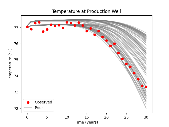
Plot prior data

The prior data show that there seem to be two possible clusters, one having slightly higher temperatures than the other. The slightly colder cluster corresponds to the models that have a connecting channel, the slightly warmer cluster the models that have no connecting channel.

fig, ax = plt.subplots()
ax.scatter(years, data_obs+k2c, label="Observed", c="r", zorder=10)
ax.plot(years, data_prior.T+k2c, c="grey", alpha=0.4,
        label=["Prior"] + [None] * (ne - 1))
ax.legend()
ax.set_xlabel("Time (years)")
ax.set_ylabel("Temperature (°C)")
ax.set_title("Temperature at Production Well")

Perform Data Assimilation (ESMDA)

# Define a function to restrict the permeability values
def restrict_permeability(x):
    """Restrict possible permeabilities."""
    np.clip(x, perm_min, perm_max, out=x)


# Run ESMDA
if compute_darts:
    perm_post, data_post = dageo.esmda(
        model_prior=perm_prior,
        forward=temperature_at_production_well,
        data_obs=data_obs,
        sigma=dstd,
        alphas=4,
        data_prior=data_prior,
        callback_post=restrict_permeability,
        random=rng,
    )

    # Store result
    np.savez_compressed(
        file="darts_output_geothermal.npz",
        data_true=data_true.astype("f"),
        data_obs=data_obs.astype("f"),
        data_prior=data_prior.astype("f"),
        data_post=data_post.astype("f"),
        perm_post=perm_post.astype("f"),
        allow_pickle=False,
    )
else:
    data_post = pc_darts["data_post"].astype("d")
    perm_post = pc_darts["perm_post"].astype("d")

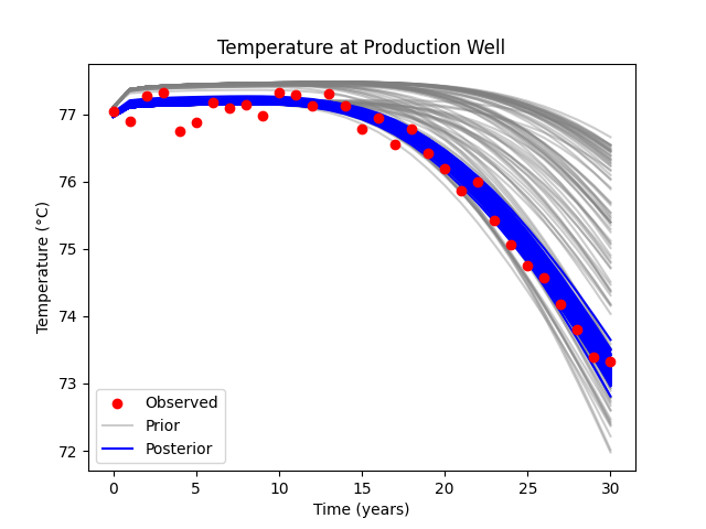
Plot posterior data

Models that connect the injection and production well with higher permeability (lower temperature) are the ones which match the data better. Even when we originally did not have channels between the injection and production well, the model found that the best way to match the data is to increase the permeability between the wells.

fig, ax = plt.subplots()
ax.scatter(years, data_obs+k2c, label="Observed", c="r", zorder=10)
ax.plot(years, data_prior.T+k2c, c="grey", alpha=0.4,
        label=["Prior"] + [None] * (ne - 1))
ax.plot(years, data_post.T+k2c, c="b",
        label=["Posterior"] + [None] * (ne - 1))
ax.legend()
ax.set_xlabel("Time (years)")
ax.set_ylabel("Temperature (°C)")
ax.set_title("Temperature at Production Well")

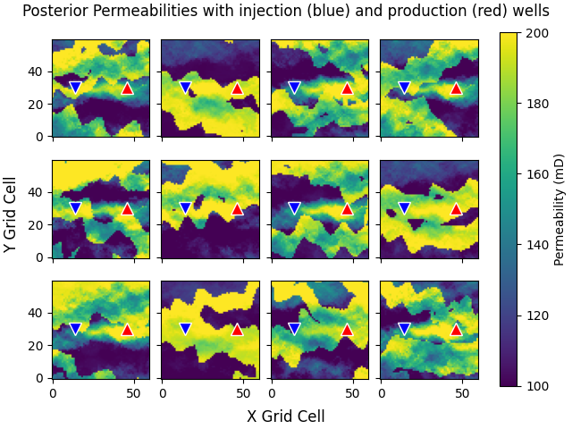
Plot posterior permeabilities

Plot the first 12 posterior permeability models.

The data is matched nicely (above figure), yet we still have different realizations, meaning that the posterior does not look like the “true” model, as expected (ill-posed problem). This means that we still have uncertainty in the model, and also that the ensemble has not collapsed to a single model.

fig, axs = plt.subplots(3, 4, **fopts)
axs = axs.ravel()
for i in range(min(ne, 12)):
    im = axs[i].imshow(perm_post[i, :, :, 0], **popts)
    axs[i].plot(jw[0], iw[0], "v", c="b", ms=10, mec="w")
    axs[i].plot(jw[1], iw[1], "^", c="r", ms=10, mec="w")
fig.colorbar(im, ax=axs, label="Permeability (mD)")
fig.suptitle(
    "Posterior Permeabilities with injection (blue) and production (red) wells"
)
fig.supylabel("Y Grid Cell")
fig.supxlabel("X Grid Cell")

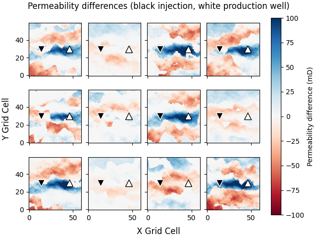
Plot permeability differences

The difference between prior and posterior shows nicely that in models, where there is a channel between the injection and production well, not much had to change in terms of permeability to predict the data. In models, however, where there is no connecting channel, it increased significantly the permeability between the wells, and decreased them further out.

popts = {"vmin": -100, "vmax": 100, "origin": "lower", "cmap": "RdBu"}
fig, axs = plt.subplots(3, 4, **fopts)
axs = axs.ravel()
for i in range(min(ne, 12)):
    im = axs[i].imshow(perm_post[i, :, :, 0] - perm_prior[i, :, :, 0], **popts)
    axs[i].plot(jw[0], iw[0], "v", c="k", ms=10, mec="w")
    axs[i].plot(jw[1], iw[1], "^", c="w", ms=10, mec="k")
fig.colorbar(im, ax=axs, label="Permeability difference (mD)")
fig.suptitle(
    "Permeability differences (black injection, white production well)"
)
fig.supylabel("Y Grid Cell")
fig.supxlabel("X Grid Cell")

Reproduce the facies

Note

The following cell is about how to reproduce the facies data loaded in facies_geothermal.nc. This was created using geomodpy.

geomodpy (Guillaume Rongier, 2023) is not open-source yet. The functionality of geomodpy that we use here is a python wrapper for the Fortran library FLUVSIM published in:

Deutsch, C. V., and T. T. Tran, 2002, FLUVSIM: a program for object-based stochastic modeling of fluvial depositional systems: Computers & Geosciences, 28(4), 525–535.

DOI: 10.1016/S0098-3004(01)00075-9.

# FLUVSIM Version used: 2.900
from geomodpy.wrapper.fluvsim import FLUVSIM

# Dimensions
nx, ny = 60, 60
dx, dy = 30, 30
ne = 100

# Create a fluvsim instance with the geological parameters
fluvsim = FLUVSIM(
    channel_orientation=(60., 90., 120.),
    # Proportions for each facies
    channel_prop=0.5,
    crevasse_prop=0.0,
    levee_prop=0.0,
    # Parameters defining the grid
    shape=(nx, ny),
    spacing=(dx, dy),
    origin=(0, 0),
    # Number of realizations and random seed
    n_realizations=ne+1,  # +1 for "true"
    seed=42,
)

# Run fluvsim to create the facies
facies = fluvsim.run()
facies = facies.data_vars["facies code"].values.astype("i4")

# Save the facies values as a compressed npy-file.
np.save("facies_geothermal.npy", facies.squeeze(), allow_pickle=False)

dageo.Report()

Fri Feb 14 07:58:30 2025 UTC
OS	Linux (Ubuntu 24.04)	CPU(s)	4	Machine	x86_64
Architecture	64bit	RAM	15.6 GiB	Environment	Python
File system	ext4
Python 3.12.9 (main, Feb 5 2025, 03:22:31) [GCC 13.3.0]
dageo	1.1.1	numpy	2.2.3	scipy	1.15.1
matplotlib	3.10.0	IPython	8.32.0

Estimated memory usage: 132 MB