Linear and non-linear ES-MDA examples

A basic example of ES-MDA using a simple 1D equation.

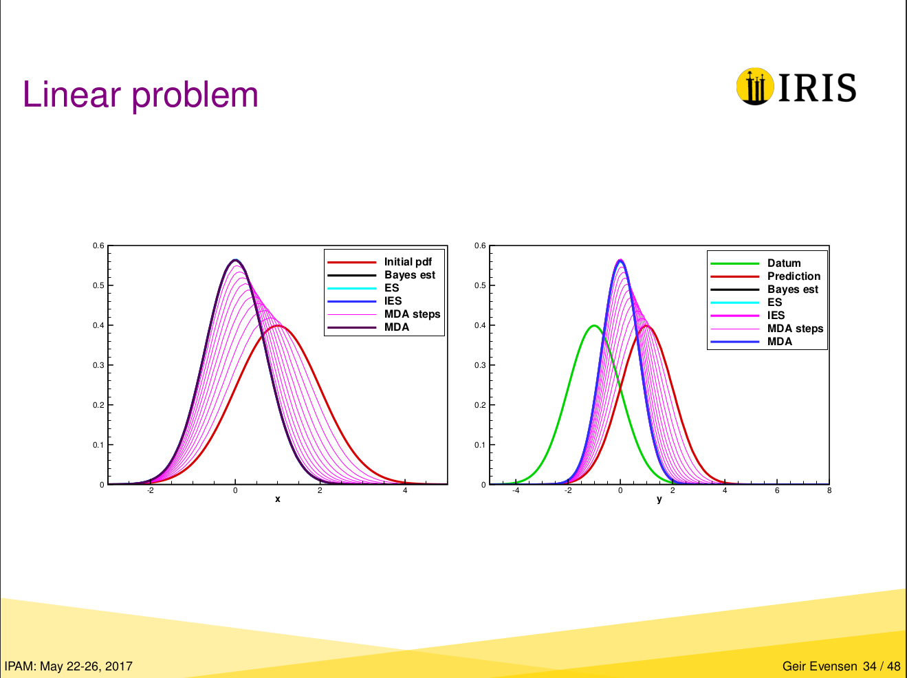
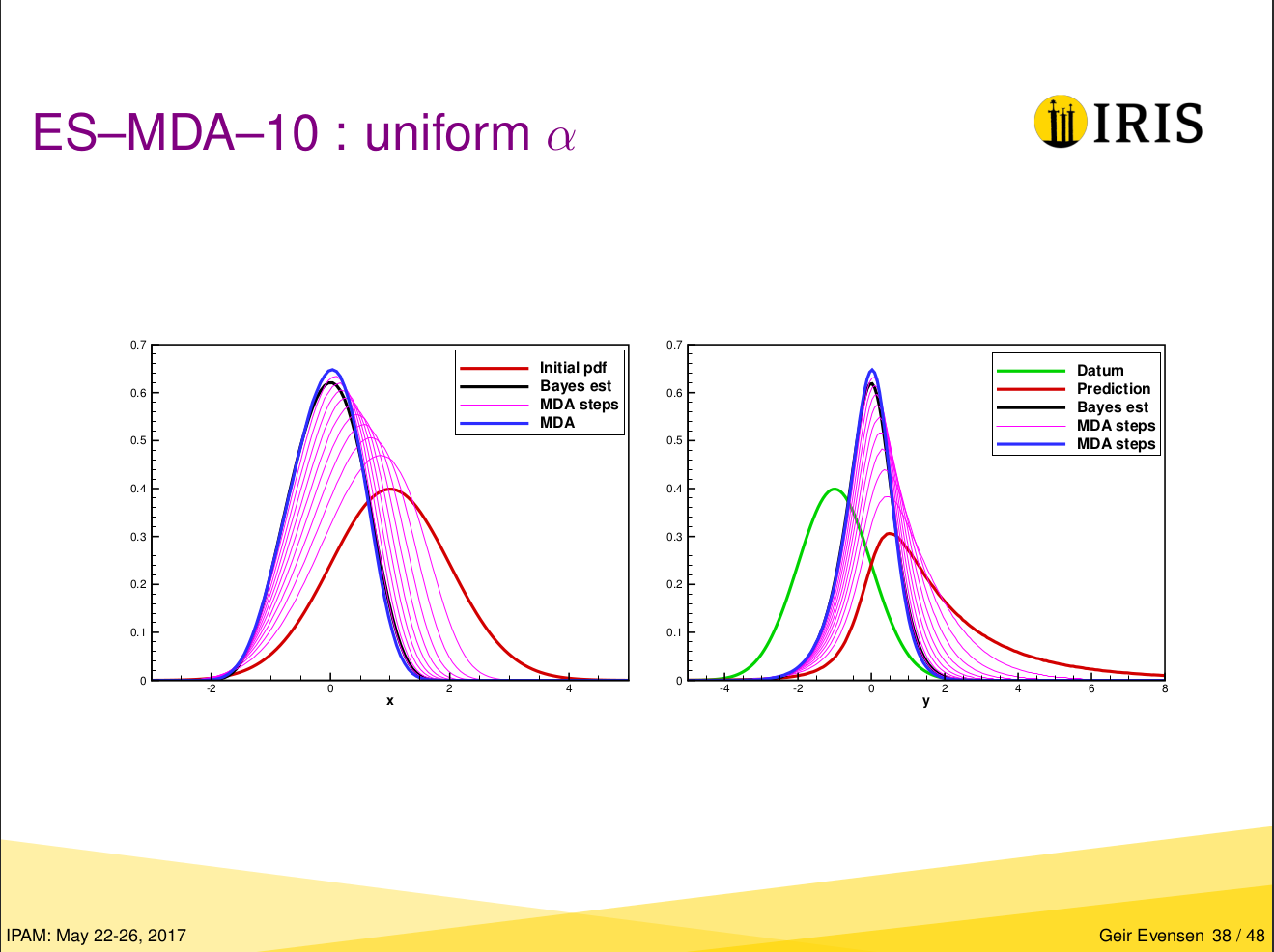
Geir Evensen gave a talk on Properties of Iterative Ensemble Smoothers and Strategies for Conditioning on Production Data at the IPAM in May 2017.

Here we reproduce the examples he showed on pages 34 and 38. The material can be found at:

• PDF: http://helper.ipam.ucla.edu/publications/oilws3/oilws3_14079.pdf

• Video can be found here: https://www.ipam.ucla.edu/programs/workshops/workshop-iii-data-assimilation-uncertainty-reduction-and-optimization-for-subsurface-flow/?tab=schedule

Geir gives the ES-MDA equations as

\[\begin{split}x_{j,i+1} &= x_{j,i} + (C^e_{xy})_i \left((C^e_{yy})_i + \alpha_iC^e_{dd}\right)^{-1} \left(d + \sqrt{\alpha_i} \varepsilon_j - g(x_{j,i})\right) \ , \\ y_{j,i+1} &= g(x_{j,i+1}) \ .\end{split}\]

The model used for this example is

\[y = x(1+\beta x^2) \ ,\]

which is a linear model if \(\beta=0\).

import numpy as np
import matplotlib.pyplot as plt

import resmda

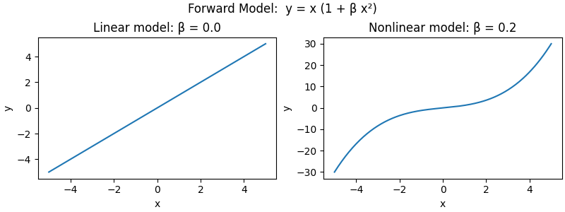
Forward model

def forward(x, beta):
    """Simple model: y = x (1 + β x²) (linear if beta=0)."""
    return np.atleast_1d(x * (1 + beta * x**2))


fig, axs = plt.subplots(
        1, 2, figsize=(8, 3), sharex=True, constrained_layout=True)
fig.suptitle("Forward Model:  y = x (1 + β x²)")
px = np.linspace(-5, 5, 301)
for i, b in enumerate([0.0, 0.2]):
    axs[i].set_title(
            f"{['Linear model', 'Nonlinear model'][i]}: β = {b}")
    axs[i].plot(px, forward(px, b))
    axs[i].set_xlabel('x')
    axs[i].set_ylabel('y')

Plotting functions

def pseudopdf(data, bins=200, density=True, **kwargs):
    """Return the pdf from a simple bin count.

    If the data contains a lot of samples, this should be "smooth" enough - and
    much faster than estimating the pdf using, e.g.,
    `scipy.stats.gaussian_kde`.
    """
    x, y = np.histogram(data, bins=bins, density=density, **kwargs)
    return (y[:-1]+y[1:])/2, x


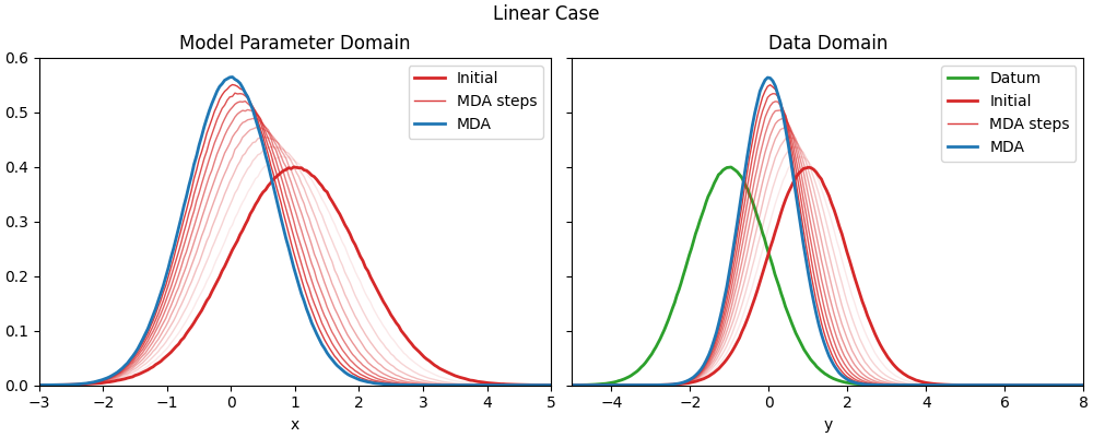
def plot_result(mpost, dpost, dobs, title, ylim):
    """Wrapper to use the same plotting for the linear and non-linear case."""

    fig, (ax1, ax2) = plt.subplots(
            1, 2, figsize=(10, 4), sharey=True, constrained_layout=True)
    fig.suptitle(title)

    # Plot Likelihood
    ax2.plot(
        *pseudopdf(resmda.rng.normal(dobs, size=(ne, dobs.size))),
        'C2', lw=2, label='Datum'
    )

    # Plot steps
    na = mpost.shape[0]-1
    for i in range(na+1):
        params = {
            'color': 'C0' if i == na else 'C3',    # Last blue, rest red
            'lw': 2 if i in [0, na] else 1,        # First/last thick
            'alpha': 1 if i in [0, na] else i/na,  # start faint
            'label': ['Initial', *((na-2)*('',)), 'MDA steps', 'MDA'][i],
        }
        ax1.plot(*pseudopdf(mpost[i, :, 0], range=(-3, 5)), **params)
        ax2.plot(*pseudopdf(dpost[i, :, 0], range=(-5, 8)), **params)

    # Axis and labels
    ax1.set_title('Model Parameter Domain')
    ax1.set_xlabel('x')
    ax1.set_ylim(ylim)
    ax1.set_xlim([-3, 5])
    ax1.legend()
    ax2.set_title('Data Domain')
    ax2.set_xlabel('y')
    ax2.set_xlim([-5, 8])
    ax2.legend()

Linear case

Prior model parameters and ES-MDA parameters

In reality, the prior would be \(j\) models provided by, e.g., the geologists. Here we create $j$ realizations using a normal distribution of a defined mean and standard deviation.

# Point of our "observation"
xlocation = -1.0

# Ensemble size
ne = int(1e7)

# Data standard deviation: ones (for this scenario)
obs_std = 1.0

# Prior: Let's start with ones as our prior guess
mprior = resmda.rng.normal(loc=1.0, scale=obs_std, size=(ne, 1))

Run ES-MDA and plot

def lin_fwd(x):
    """Linear forward model."""
    return forward(x, beta=0.0)


# Sample an "observation".
l_dobs = lin_fwd(xlocation)

lm_post, ld_post = resmda.esmda(
    model_prior=mprior,
    forward=lin_fwd,
    data_obs=l_dobs,
    sigma=obs_std,
    alphas=10,
    return_steps=True,  # To get intermediate results
)

ES-MDA step   1; α=10.0
ES-MDA step   2; α=10.0
ES-MDA step   3; α=10.0
ES-MDA step   4; α=10.0
ES-MDA step   5; α=10.0
ES-MDA step   6; α=10.0
ES-MDA step   7; α=10.0
ES-MDA step   8; α=10.0
ES-MDA step   9; α=10.0
ES-MDA step  10; α=10.0

plot_result(lm_post, ld_post, l_dobs, title='Linear Case', ylim=[0, 0.6])

Original figure from Geir’s presentation

Nonlinear case

def nonlin_fwd(x):
    """Nonlinear forward model."""
    return forward(x, beta=0.2)


# Sample a nonlinear observation; the rest of the parameters remains the same.
n_dobs = nonlin_fwd(xlocation)
nm_post, nd_post = resmda.esmda(
    model_prior=mprior,
    forward=nonlin_fwd,
    data_obs=n_dobs,
    sigma=obs_std,
    alphas=10,
    return_steps=True,
)

ES-MDA step   1; α=10.0
ES-MDA step   2; α=10.0
ES-MDA step   3; α=10.0
ES-MDA step   4; α=10.0
ES-MDA step   5; α=10.0
ES-MDA step   6; α=10.0
ES-MDA step   7; α=10.0
ES-MDA step   8; α=10.0
ES-MDA step   9; α=10.0
ES-MDA step  10; α=10.0

plot_result(nm_post, nd_post, n_dobs, title='Nonlinear Case', ylim=[0, 0.7])

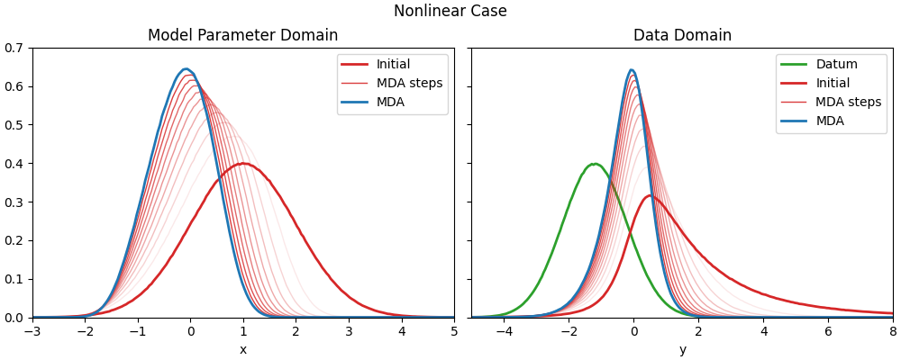
Original figure from Geir’s presentation

resmda.Report()

Wed Jul 24 14:03:58 2024 UTC
OS	Linux (Ubuntu 22.04)	CPU(s)	4	Machine	x86_64
Architecture	64bit	RAM	15.6 GiB	Environment	Python
File system	ext4
Python 3.11.9 (main, Jul 15 2024, 21:50:21) [GCC 11.4.0]
numpy	2.0.1	scipy	1.14.0	numba	Module not found
resmda	0.2.0	matplotlib	3.9.1	IPython	8.26.0