2D Fluvial Reservoir ESMDA example

In contrast to the basic reservoir example 2D Reservoir ESMDA example, where a single facies was used, this example uses fluvial models containing different facies. It also compares the use of ES-MDA with and without localization, as explained in the example Localization.

The fluvial models were generated with FLUVSIM through geomodpy, for more information see towards the end of the example where the code is shown to reproduce the facies.

Note

To retrieve the data, you need to have pooch installed:

pip install pooch

or

conda install -c conda-forge pooch

import os
import json

import pooch
import numpy as np
import matplotlib.pyplot as plt

import resmda

# For reproducibility, we instantiate a random number generator with a fixed
# seed. For production, remove the seed!
rng = np.random.default_rng(1513)

# Adjust this path to a folder of your choice.
data_path = os.path.join("..", "download", "")

Load and plot the facies

fname = "facies.npy"
pooch.retrieve(
    "https://raw.github.com/tuda-geo/data/2024-06-18/resmda/"+fname,
    "4bfe56c836bf17ca63453c37e5da91cb97bbef8cc6c08d605f70bd64fe7488b2",
    fname=fname,
    path=data_path,
)
facies = np.load(data_path + fname)
ne, nx, ny = facies.shape

# Define mean permeability per facies
perm_means = [0.1, 5.0, 3.0]

# Plot the facies
fig, axs = plt.subplots(
    2, 5, figsize=(8, 3), sharex=True, sharey=True, constrained_layout=True)
axs = axs.ravel()
fig.suptitle(f"Facies {[f'{i} = {p}' for i, p in enumerate(perm_means)]}")
for i in range(ne):
    im = axs[i].imshow(
        facies[i, ...], cmap=plt.get_cmap("Accent", 3),
        clim=[-0.5, 2.5], origin="lower"
    )
fig.colorbar(im, ax=axs, ticks=[0, 1, 2], label="Facies code")

Downloading data from 'https://raw.github.com/tuda-geo/data/2024-06-18/resmda/facies.npy' to file '/home/runner/work/resmda/resmda/download/facies.npy'.

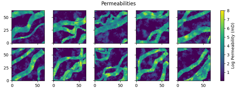
Assign random permeabilities to the facies

perm_min = 0.05
perm_max = 10.0

# Instantiate a random permeability instance
RP = resmda.RandomPermeability(
    nx, ny, perm_mean=None, perm_min=perm_min, perm_max=perm_max
)

# Fill the different facies with their permeabilities
permeabilities = np.empty(facies.shape)
for code, mean in enumerate(perm_means):
    mask = facies == code
    permeabilities[mask] = RP(ne, perm_mean=mean)[mask]

fig, axs = plt.subplots(
    2, 5, figsize=(8, 3), sharex=True, sharey=True, constrained_layout=True)
axs = axs.ravel()
fig.suptitle("Permeabilities")
for i in range(ne):
    im = axs[i].imshow(permeabilities[i, ...], origin="lower")
fig.colorbar(im, ax=axs, label="Log Permeability (mD)")

Model parameters

# We take the first model as "true/reference", and the other for ES-MDA.
perm_true = permeabilities[0, ...][None, ...]
perm_prior = permeabilities[1:, ...]

# Time steps
dt = np.zeros(10)+0.0001
time = np.r_[0, np.cumsum(dt)]
nt = time.size

# Assumed standard deviation of our data
dstd = 0.5

# Measurement points
ox = (5, 15, 24)
oy = (5, 10, 24)

# Number of data points
nd = time.size * len(ox)

# Wells
wells = np.array([
    [ox[0], oy[0], 180], [5, 12, 120],
    [ox[1], oy[1], 180], [20, 5, 120],
    [ox[2], oy[2], 180], [24, 17, 120]
])

Run the prior models and the reference case

# Instantiate reservoir simulator
RS = resmda.Simulator(nx, ny, wells=wells)


def sim(x):
    """Custom fct to use exp(x), and specific dt & location."""
    return RS(np.exp(x), dt=dt, data=(ox, oy)).reshape((x.shape[0], -1))


# Simulate data for the prior and true fields
data_prior = sim(perm_prior)
data_true = sim(perm_true)
data_obs = rng.normal(data_true, dstd)
data_obs[0, :3] = data_true[0, :3]

Localization Matrix

# Vector of nd length with the well x and y position for each nd data point
nd_positions = np.tile(np.array([ox, oy]), time.size).T

# Create matrix
loc_mat = resmda.localization_matrix(RP.cov, nd_positions, (nx, ny))

ES-MDA

def restrict_permeability(x):
    """Restrict possible permeabilities."""
    np.clip(x, perm_min, perm_max, out=x)


inp = {
    "model_prior": perm_prior,
    "forward": sim,
    "data_obs": data_obs,
    "sigma": dstd,
    "alphas": 4,
    "data_prior": data_prior,
    "callback_post": restrict_permeability,
    "random": rng,
}

Without localization

nl_perm_post, nl_data_post = resmda.esmda(**inp)

ES-MDA step   1; α=4.0
ES-MDA step   2; α=4.0
ES-MDA step   3; α=4.0
ES-MDA step   4; α=4.0

With localization

wl_perm_post, wl_data_post = resmda.esmda(**inp, localization_matrix=loc_mat)

ES-MDA step   1; α=4.0
ES-MDA step   2; α=4.0
ES-MDA step   3; α=4.0
ES-MDA step   4; α=4.0

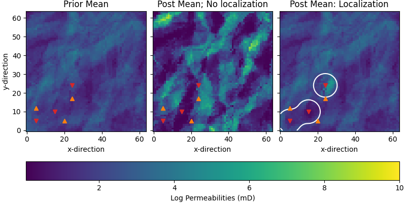
Compare permeabilities

# Plot posterior
fig, axs = plt.subplots(
    1, 3, figsize=(8, 4), sharex=True, sharey=True, constrained_layout=True)

par = {"vmin": perm_min, "vmax": perm_max, "origin": "lower"}

axs[0].set_title("Prior Mean")
im = axs[0].imshow(perm_prior.mean(axis=0).T, **par)


axs[1].set_title("Post Mean; No localization")
axs[1].imshow(nl_perm_post.mean(axis=0).T, **par)

axs[2].set_title("Post Mean: Localization")
axs[2].imshow(wl_perm_post.mean(axis=0).T, **par)
axs[2].contour(loc_mat.sum(axis=2).T, levels=[2.0, ], colors="w")

fig.colorbar(im, ax=axs, label="Log Permeabilities (mD)",
             orientation="horizontal")

for ax in axs:
    for well in wells:
        ax.plot(well[0], well[1], ["C3v", "C1^"][int(well[2] == 120)])
for ax in axs:
    ax.set_xlabel('x-direction')
axs[0].set_ylabel('y-direction')

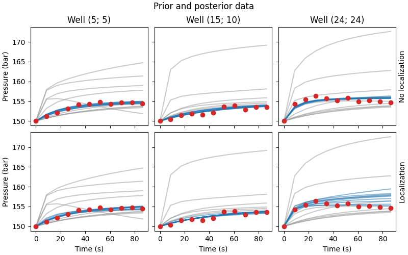
Compare data

# QC data and priors
fig, axs = plt.subplots(
    2, 3, figsize=(8, 5), sharex=True, sharey=True, constrained_layout=True)
fig.suptitle("Prior and posterior data")
for i, ax in enumerate(axs[0, :]):
    ax.set_title(f"Well ({ox[i]}; {oy[i]})")
    ax.plot(time*24*60*60, data_prior[..., i::3].T, color=".6", alpha=0.5)
    ax.plot(time*24*60*60, nl_data_post[..., i::3].T, color="C0", alpha=0.5)
    ax.plot(time*24*60*60, data_obs[0, i::3], "C3o")
for i, ax in enumerate(axs[1, :]):
    ax.plot(time*24*60*60, data_prior[..., i::3].T, color=".6", alpha=0.5)
    ax.plot(time*24*60*60, wl_data_post[..., i::3].T, color="C0", alpha=0.5)
    ax.plot(time*24*60*60, data_obs[0, i::3], "C3o")
    ax.set_xlabel("Time (s)")
for i, ax in enumerate(axs[:, 0]):
    ax.set_ylabel("Pressure (bar)")
for i, txt in enumerate(["No l", "L"]):
    axs[i, 2].yaxis.set_label_position("right")
    axs[i, 2].set_ylabel(f"{txt}ocalization")

Reproduce the facies

Note

The following cell is about how to reproduce the facies data loaded in facies.npy. This was created using geomodpy.

geomodpy (Guillaume Rongier, 2023) is not open-source yet. The functionality of geomodpy that we use here is a python wrapper for the Fortran library FLUVSIM published in:

Deutsch, C. V., and T. T. Tran, 2002, FLUVSIM: a program for object-based stochastic modeling of fluvial depositional systems: Computers & Geosciences, 28(4), 525–535.

DOI: 10.1016/S0098-3004(01)00075-9.

# ==== Required imports ====
import json
import numpy as np

# FLUVSIM Version used: 2.900
from geomodpy.wrapper.fluvsim import FLUVSIM

# For reproducibility, we instantiate a random number generator with a
# fixed seed. For production, remove the seed!
rng = np.random.default_rng(1848)


# ==== Define the geological parameters ====

# Here we define the geological parameters by means of their normal
# distribution parameters

# Each tuple stands for (mean, std); lists contain several of them.
geol_distributions = {
    "channel_orientation": (60, 20),
    "channel_amplitude": [(100, 1), (250, 1), (400, 1)],
    "channel_wavelength": [(1000, 5), (2000, 5), (3000, 5)],
    "channel_thickness": [(4, 0.1), (8, 0.1), (11, 0.1)],
    "channel_thickness_undulation": (1, 0.02),
    "channel_thickness_undulation_wavelength": [
        (250, 1), (400, 1), (450, 1)
    ],
    "channel_width_thickness_ratio": [(40, 0.5), (50, 0.5), (60, 0.5)],
    "channel_width_undulation": (1, 0.02),
    "channel_width_undulation_wavelength": (250, 1),
    "channel_prop": (0.4, 0.005),
}


def generate_geol_params(geol_dists):
    """Generate geological parameters from normal distributions.

    Expects for each parameter a tuple of two values, or a list
    containing tuples of two values each.
    """
    geol_params = {}
    for param, dist in geol_dists.items():
        if isinstance(dist, list):
            geol_params[param] = tuple(
                rng.normal(mean, std) for mean, std in dist
            )
        else:
            geol_params[param] = rng.normal(*dist)
    return geol_params


# ==== Create the facies ====

# Number of sets and realizations
nsets = 2
nreal = 5

# Model dimension
nx, ny, nz = 64, 64, 1

# Pre-allocate containers to store all realizations and their
# corresponding parameters
all_params = {}
facies = np.zeros((nsets * nreal, nz, nx, ny), dtype="i4")

for i in range(nsets):  # We create two sets
    print(f"Generating realization {i+1} of {nsets}")

    params = generate_geol_params(geol_distributions)
    all_params[f"set-{i}"] = params

    fluvsim = FLUVSIM(
        shape=(nx, ny, nz),
        spacing=(50, 50, 1),
        origin=(25, 25, 0.5),
        n_realizations=nreal,
        **params
    )

    realizations = fluvsim.run().data_vars["facies code"].values
    facies[i*nreal:(i+1)*nreal, ...] = realizations.astype("i4")


# ==== Save the output ====

# Save the input parameters to FLUVSIM as a json.
with open("facies.json", "w") as f:
    json.dump(all_params, f, indent=2)
# Save the facies values as a compressed npy-file.
np.save("facies", facies.squeeze(), allow_pickle=False)

Input parameters to FLUVSIM

For reproducibility purposes we print here the used input values to FLUVSIM. These are, just as the data themselves, online at tuda-geo/data.

fname = "facies.json"
pooch.retrieve(
    "https://raw.github.com/tuda-geo/data/2024-06-18/resmda/"+fname,
    "db2cb8a620775c68374c24a4fa811f6350381c7fc98a823b9571136d307540b4",
    fname=fname,
    path=data_path,
)
with open(data_path + fname, "r") as f:
    print(json.dumps(json.load(f), indent=2))

Downloading data from 'https://raw.github.com/tuda-geo/data/2024-06-18/resmda/facies.json' to file '/home/runner/work/resmda/resmda/download/facies.json'.
{
  "set-0": {
    "channel_orientation": 63.93933122172756,
    "channel_amplitude": [
      99.72003201597424,
      250.09738942599537,
      399.99645679311095
    ],
    "channel_wavelength": [
      998.3771346070469,
      2006.0222525108188,
      3002.013904724877
    ],
    "channel_thickness": [
      4.015660555164119,
      8.02125812391539,
      10.807448731138143
    ],
    "channel_thickness_undulation": 1.006385274247584,
    "channel_thickness_undulation_wavelength": [
      250.36201979679302,
      398.4759608983245,
      448.44486265914315
    ],
    "channel_width_thickness_ratio": [
      40.545201273906024,
      50.53224723965168,
      60.21913791333122
    ],
    "channel_width_undulation": 1.021202467139173,
    "channel_width_undulation_wavelength": 249.2684837598085,
    "channel_prop": 0.40189379634538847
  },
  "set-1": {
    "channel_orientation": 45.94027637621462,
    "channel_amplitude": [
      98.16203534405199,
      251.1448878929924,
      400.3245308818956
    ],
    "channel_wavelength": [
      1009.8934540579546,
      2008.4295824697977,
      3003.9136764267087
    ],
    "channel_thickness": [
      4.111706626685296,
      8.002547496480005,
      10.775694168554176
    ],
    "channel_thickness_undulation": 1.0147354365869505,
    "channel_thickness_undulation_wavelength": [
      249.9803344958115,
      398.8015770326054,
      448.3657322896644
    ],
    "channel_width_thickness_ratio": [
      39.87761151661253,
      49.4521315931951,
      58.02613825217046
    ],
    "channel_width_undulation": 0.9945245219176657,
    "channel_width_undulation_wavelength": 250.56212687685527,
    "channel_prop": 0.4022891542425987
  }
}

resmda.Report()

Wed Jul 24 14:04:21 2024 UTC
OS	Linux (Ubuntu 22.04)	CPU(s)	4	Machine	x86_64
Architecture	64bit	RAM	15.6 GiB	Environment	Python
File system	ext4
Python 3.11.9 (main, Jul 15 2024, 21:50:21) [GCC 11.4.0]
numpy	2.0.1	scipy	1.14.0	numba	Module not found
resmda	0.2.0	matplotlib	3.9.1	IPython	8.26.0