Localization

This example follows contextually 2D Reservoir ESMDA example, but uses several well doublets and compares ES-MDA with and without localization.

import numpy as np
import matplotlib.pyplot as plt

import resmda

# For reproducibility, we instantiate a random number generator with a fixed
# seed. For production, remove the seed!
rng = np.random.default_rng(2020)

Model parameters

# Grid extension
nx = 35
ny = 30
nc = nx*ny

# Permeabilities
perm_mean = 3.0
perm_min = 0.5
perm_max = 5.0

# ESMDA parameters
ne = 100                  # Number of ensembles
dt = np.zeros(10)+0.0001  # Time steps (could be irregular, e.g., increasing!)
time = np.r_[0, np.cumsum(dt)]

# Assumed sandard deviation of our data
dstd = 0.5

# Measurement points
ox = (5, 15, 24)
oy = (5, 10, 24)

# Number of data points
nd = time.size * len(ox)

# Wells
wells = np.array([
    [ox[0], oy[0], 180], [5, 12, 120],
    [ox[1], oy[1], 180], [20, 5, 120],
    [ox[2], oy[2], 180], [24, 17, 120]
])

Create permeability maps for ESMDA

We will create a set of permeability maps that will serve as our initial guess (prior). These maps are generated using a Gaussian random field and are constrained by certain statistical properties.

# Get the model and ne prior models
RP = resmda.RandomPermeability(nx, ny, perm_mean, perm_min, perm_max)
perm_true = RP(1, random=rng)
perm_prior = RP(ne, random=rng)

Run the prior models and the reference case

# Instantiate reservoir simulator
RS = resmda.Simulator(nx, ny, wells=wells)


def sim(x):
    """Custom fct to use exp(x), and specific dt & location."""
    return RS(np.exp(x), dt=dt, data=(ox, oy)).reshape((x.shape[0], -1))


# Simulate data for the prior and true fields
data_prior = sim(perm_prior)
data_true = sim(perm_true)
data_obs = rng.normal(data_true, dstd)
data_obs[0, :3] = data_true[0, :3]

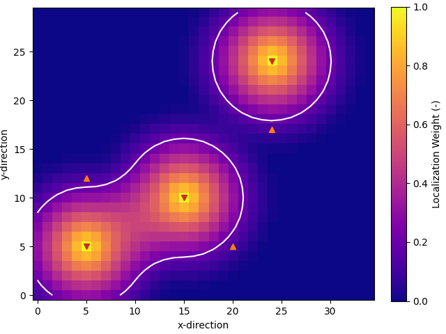
Localization Matrix

# Vector of nd length with the well x and y position for each nd data point
nd_positions = np.tile(np.array([ox, oy]), time.size).T

# Create matrix
loc_mat = resmda.localization_matrix(RP.cov, nd_positions, (nx, ny))

# QC localization matrix
fig, ax = plt.subplots(1, 1, constrained_layout=True)
im = ax.imshow(loc_mat.sum(axis=2).T/time.size, origin='lower', cmap="plasma")
ax.contour(loc_mat.sum(axis=2).T/time.size, levels=[0.2, ], colors='w')
ax.set_xlabel('x-direction')
ax.set_ylabel('y-direction')
for well in wells:
    ax.plot(well[0], well[1], ['C3v', 'C1^'][int(well[2] == 120)])
fig.colorbar(im, ax=ax, label="Localization Weight (-)")

ES-MDA

def restrict_permeability(x):
    """Restrict possible permeabilities."""
    np.clip(x, perm_min, perm_max, out=x)


inp = {
    'model_prior': perm_prior,
    'forward': sim,
    'data_obs': data_obs,
    'sigma': dstd,
    'alphas': 4,
    'data_prior': data_prior,
    'callback_post': restrict_permeability,
    'random': rng,
}

Without localization

nl_perm_post, nl_data_post = resmda.esmda(**inp)

ES-MDA step   1; α=4.0
ES-MDA step   2; α=4.0
ES-MDA step   3; α=4.0
ES-MDA step   4; α=4.0

With localization

wl_perm_post, wl_data_post = resmda.esmda(**inp, localization_matrix=loc_mat)

ES-MDA step   1; α=4.0
ES-MDA step   2; α=4.0
ES-MDA step   3; α=4.0
ES-MDA step   4; α=4.0

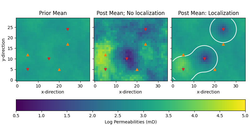
Compare permeabilities

# Plot posterior
fig, axs = plt.subplots(
    1, 3, figsize=(8, 4), sharex=True, sharey=True, constrained_layout=True)

par = {"vmin": perm_min, "vmax": perm_max, "origin": "lower"}

axs[0].set_title("Prior Mean")
im = axs[0].imshow(perm_prior.mean(axis=0).T, **par)


axs[1].set_title("Post Mean; No localization")
axs[1].imshow(nl_perm_post.mean(axis=0).T, **par)

axs[2].set_title("Post Mean: Localization")
axs[2].imshow(wl_perm_post.mean(axis=0).T, **par)
axs[2].contour(loc_mat.sum(axis=2).T, levels=[2.0, ], colors="w")

fig.colorbar(im, ax=axs, label="Log Permeabilities (mD)",
             orientation="horizontal")

for ax in axs:
    for well in wells:
        ax.plot(well[0], well[1], ["C3v", "C1^"][int(well[2] == 120)])
for ax in axs:
    ax.set_xlabel('x-direction')
axs[0].set_ylabel('y-direction')

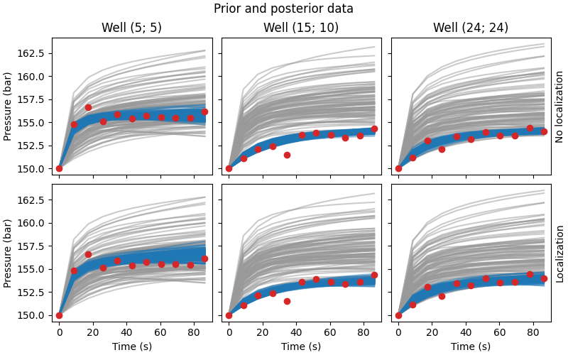
Compare data

# QC data and priors
fig, axs = plt.subplots(
    2, 3, figsize=(8, 5), sharex=True, sharey=True, constrained_layout=True)
fig.suptitle('Prior and posterior data')
for i, ax in enumerate(axs[0, :]):
    ax.set_title(f"Well ({ox[i]}; {oy[i]})")
    ax.plot(time*24*60*60, data_prior[..., i::3].T, color='.6', alpha=0.5)
    ax.plot(time*24*60*60, nl_data_post[..., i::3].T, color='C0', alpha=0.5)
    ax.plot(time*24*60*60, data_obs[0, i::3], 'C3o')
for i, ax in enumerate(axs[1, :]):
    ax.plot(time*24*60*60, data_prior[..., i::3].T, color='.6', alpha=0.5)
    ax.plot(time*24*60*60, wl_data_post[..., i::3].T, color='C0', alpha=0.5)
    ax.plot(time*24*60*60, data_obs[0, i::3], 'C3o')
    ax.set_xlabel("Time (s)")
for i, ax in enumerate(axs[:, 0]):
    ax.set_ylabel("Pressure (bar)")
for i, txt in enumerate(["No l", "L"]):
    axs[i, 2].yaxis.set_label_position("right")
    axs[i, 2].set_ylabel(f"{txt}ocalization")

resmda.Report()

Wed Jul 24 14:04:40 2024 UTC
OS	Linux (Ubuntu 22.04)	CPU(s)	4	Machine	x86_64
Architecture	64bit	RAM	15.6 GiB	Environment	Python
File system	ext4
Python 3.11.9 (main, Jul 15 2024, 21:50:21) [GCC 11.4.0]
numpy	2.0.1	scipy	1.14.0	numba	Module not found
resmda	0.2.0	matplotlib	3.9.1	IPython	8.26.0