2D Reservoir ESMDA example

Ensemble Smoother Multiple Data Assimilation (ES-MDA) in Reservoir Simulation.

import numpy as np
import matplotlib.pyplot as plt

import resmda

# For reproducibility, we instantiate a random number generator with a fixed
# seed. For production, remove the seed!
rng = np.random.default_rng(1848)

Model parameters

# Grid extension
nx = 30
ny = 25
nc = nx*ny

# Permeabilities
perm_mean = 3.0
perm_min = 0.5
perm_max = 5.0

# ESMDA parameters
ne = 100                  # Number of ensembles
dt = np.zeros(10)+0.0001  # Time steps (could be irregular, e.g., increasing!)
time = np.r_[0, np.cumsum(dt)]
nt = time.size

# Assumed sandard deviation of our data
dstd = 0.5

# Observation location indices (should be well locations)
ox, oy = 1, 1

# Wells (if None, first and last cells are used with pressure 180 and 120)
wells = None

Create permeability maps for ESMDA

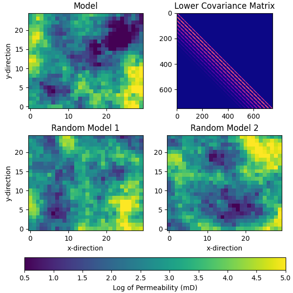
We will create a set of permeability maps that will serve as our initial guess (prior). These maps are generated using a Gaussian random field and are constrained by certain statistical properties.

# Get the model and ne prior models
RP = resmda.RandomPermeability(nx, ny, perm_mean, perm_min, perm_max)
perm_true = RP(1, random=rng)
perm_prior = RP(ne, random=rng)


# QC covariance, reference model, and first two random models
pinp1 = {"origin": "lower", "vmin": perm_min, "vmax": perm_max}
fig, axs = plt.subplots(2, 2, figsize=(6, 6), constrained_layout=True)
axs[0, 0].set_title("Model")
im = axs[0, 0].imshow(perm_true.T, **pinp1)
axs[0, 1].set_title("Lower Covariance Matrix")
im2 = axs[0, 1].imshow(RP.cov, cmap="plasma")
axs[1, 0].set_title("Random Model 1")
axs[1, 0].imshow(perm_prior[0, ...].T, **pinp1)
axs[1, 1].set_title("Random Model 2")
axs[1, 1].imshow(perm_prior[1, ...].T, **pinp1)
fig.colorbar(im, ax=axs[1, :], orientation="horizontal",
             label="Log of Permeability (mD)")
for ax in axs[1, :].ravel():
    ax.set_xlabel("x-direction")
for ax in axs[:, 0].ravel():
    ax.set_ylabel("y-direction")

Run the prior models and the reference case

# Instantiate reservoir simulator
RS = resmda.Simulator(nx, ny, wells=wells)


def sim(x):
    """Custom fct to use exp(x), and specific dt & location."""
    return RS(np.exp(x), dt=dt, data=(ox, oy))


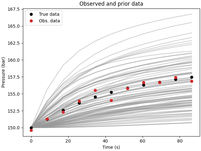
# Simulate data for the prior and true fields
data_prior = sim(perm_prior)
data_true = sim(perm_true)
data_obs = rng.normal(data_true, dstd)

# QC data and priors
fig, ax = plt.subplots(1, 1, constrained_layout=True)
ax.set_title("Observed and prior data")
ax.plot(time*24*60*60, data_prior.T, color=".6", alpha=0.5)
ax.plot(time*24*60*60, data_true, "ko", label="True data")
ax.plot(time*24*60*60, data_obs, "C3o", label="Obs. data")
ax.legend()
ax.set_xlabel("Time (s)")
ax.set_ylabel("Pressure (bar)")

ESMDA

def restrict_permeability(x):
    """Restrict possible permeabilities."""
    np.clip(x, perm_min, perm_max, out=x)


perm_post, data_post = resmda.esmda(
    model_prior=perm_prior,
    forward=sim,
    data_obs=data_obs,
    sigma=dstd,
    alphas=4,
    data_prior=data_prior,
    callback_post=restrict_permeability,
    random=rng,
)

ES-MDA step   1; α=4.0
ES-MDA step   2; α=4.0
ES-MDA step   3; α=4.0
ES-MDA step   4; α=4.0

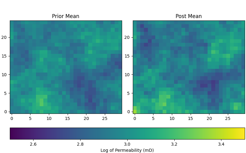
Posterior Analysis

After running ESMDA, it’s crucial to analyze the posterior ensemble of models. Here, we visualize the first three realizations from both the prior and posterior ensembles to see how the models have been updated.

# Plot posterior
fig, ax = plt.subplots(1, 2, figsize=(8, 5), constrained_layout=True)
pinp2 = {"origin": "lower", "vmin": 2.5, "vmax": 3.5}
ax[0].set_title("Prior Mean")
im = ax[0].imshow(perm_prior.mean(axis=0).T, **pinp2)
ax[1].set_title("Post Mean")
ax[1].imshow(perm_post.mean(axis=0).T, **pinp2)
fig.colorbar(im, ax=ax, label="Log of Permeability (mD)",
             orientation="horizontal")

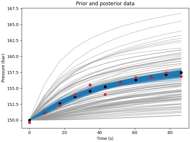
Observing the monitored pressure at cell (1,1) for all realizations and the reference case, we can see that the ensemble of models after the assimilation steps (in blue) is closer to the reference case (in red) than the prior ensemble (in gray). This indicates that the ESMDA method is effectively updating the models to better represent the observed data.

# Compare posterior to prior and observed data
fig, ax = plt.subplots(1, 1, constrained_layout=True)
ax.set_title("Prior and posterior data")
ax.plot(time*24*60*60, data_prior.T, color=".6", alpha=0.5)
ax.plot(time*24*60*60, data_post.T, color="C0", alpha=0.5)
ax.plot(time*24*60*60, data_true, "ko")
ax.plot(time*24*60*60, data_obs, "C3o")
ax.set_xlabel("Time (s)")
ax.set_ylabel("Pressure (bar)")

resmda.Report()

Wed Jul 24 14:04:06 2024 UTC
OS	Linux (Ubuntu 22.04)	CPU(s)	4	Machine	x86_64
Architecture	64bit	RAM	15.6 GiB	Environment	Python
File system	ext4
Python 3.11.9 (main, Jul 15 2024, 21:50:21) [GCC 11.4.0]
numpy	2.0.1	scipy	1.14.0	numba	Module not found
resmda	0.2.0	matplotlib	3.9.1	IPython	8.26.0